What is Fuzzy Lookup Function in Excel?

Fuzzy Lookup Function is used to lookup two tables that have similar data but with minor differences, such as a spelling error. All the lookup functions in Excel, perform only when there is exact match between two sets of Data. Often, people make mistakes while preparing data such as instead of using the database code or naming convention, they manually type the name which results in slight difference between the name store in the database. To correct the data error, you must go through a cumbersome process of looking at each mistake and correcting it. We can easily compare data that has minor changes by the help of Fuzzy Lookup Function in Excel.

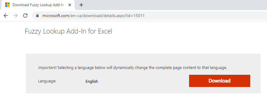
It comes in the form of external add-in which is available on Microsoft Website and it can be downloaded for the link “https://www.microsoft.com/en-ca/download/details.aspx?id=15011” .

Practical applications of Fuzzy Lookup Function in Excel

Example 

We are using a sample database file that contains item code and item names. We want to upload the revision of prices to our Database and we have prices in a different sheet but the item names on that sheet have some spelling error due to which the lookup functions will return an error. Therefore, we will use the Fuzzy Lookup Function to compare the two tables side by side.

Step 1: Go to the Link: https://www.microsoft.com/en-ca/download/details.aspx?id=15011 and download the Fuzzy Lookup Add-in.

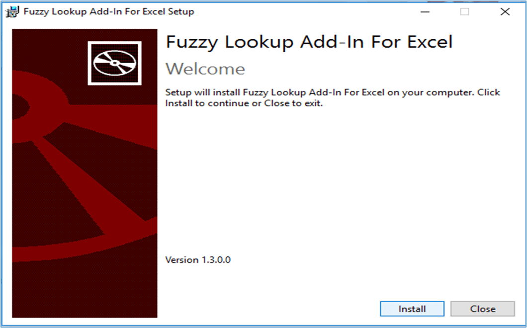
Step 2:  An installation window will open, install the add-in from there. When you open the next instance of Microsoft Excel, the Fuzzy Lookup Tab will automatically appear in the Main Tabs.

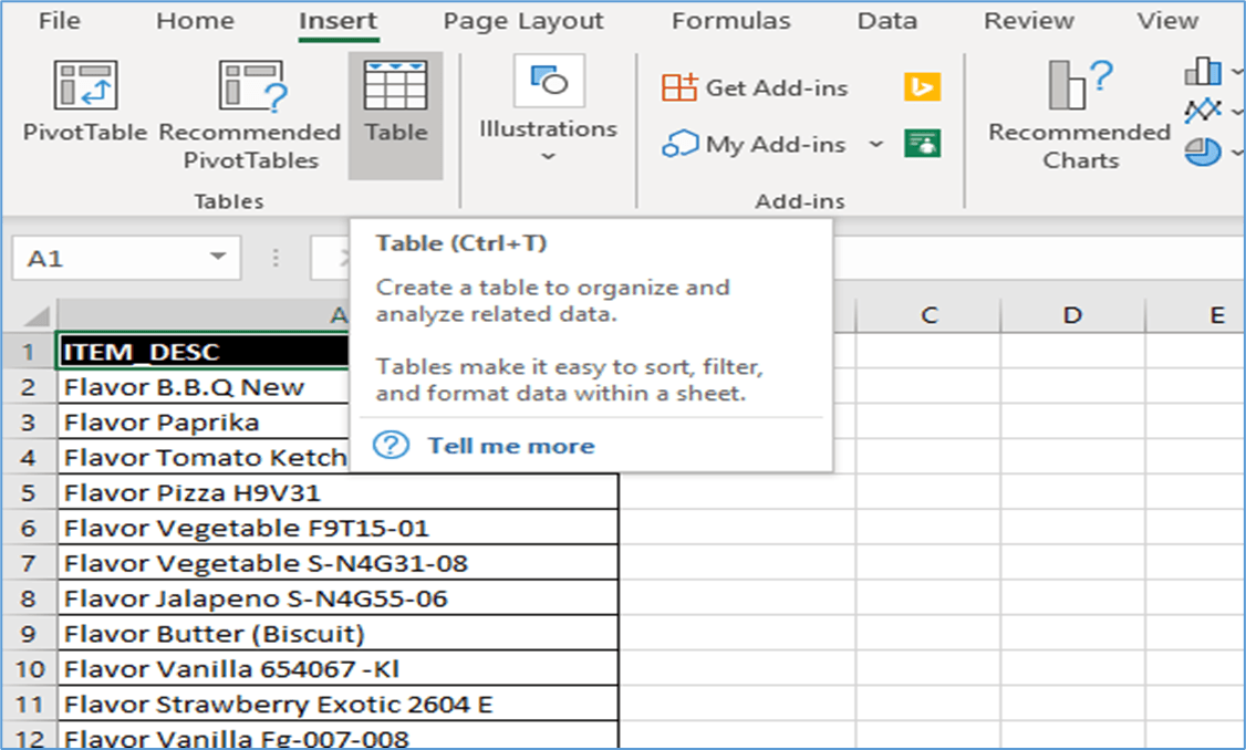
Step 3: Copy your Database item names and price list item names in separate sheets in Column A. Then convert both lists in separate worksheets into Tables. To convert the lists into tables, Go to Insert Tab > Table. A create table window will appear. Click Ok to convert the list into Table. The reason for doing this is to instruct Excel to perform the Fuzzy Lookup Function on the table rather than on a particular cell.

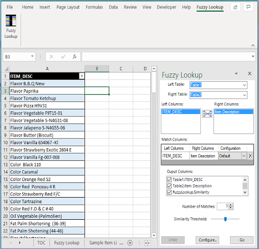
Step 4: Navigate to Fuzzy Lookup from the Fuzzy Lookup Tab. A window will appear to your right. Read through it and select the following according to your need.
(i) Select number of matches as one if you want the match to return the closest match. Otherwise you can change this for multiple matches.
(ii) Select the similarity threshold according to the level of accuracy you want the data to be in. It is a good practice to use sensitivity of 0.9-1.0 as this will give more accurate results.

Step 5: The result will be as shown below. The Fuzzy Lookup Function will compare both Tables and show the Similarity threshold between both list items. You can now use this as a reference point for your workings. To get the prices against the database item names, simply use the VLOOKUP function on the database item names and copy the corresponding price list item names from the Fuzzy Lookup comparison sheet. Then use the price list item names that were copied with the VLOOKUP function and again use it to VLOOKUP the Prices from the Price List.

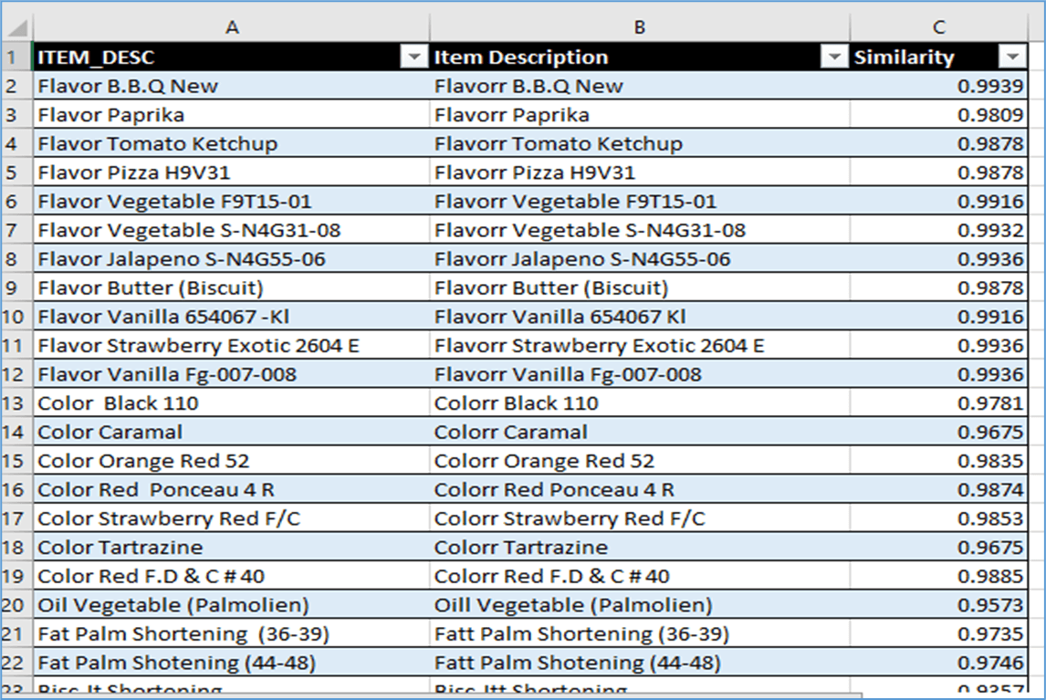
Now that you understand how the Fuzzy Lookup Function works, you can use it to compare any set of data that contains minor errors. You might also have data that have multiple error for the same name and for that purpose you can set the Match to more than 1 as explained in Part Four of Step Four. You can experiment and work around the Fuzzy Lookup Function-in to get a better idea of how it can be suited to your needs.

I hope that helps. Please leave a comment below with any questions or suggestions. For more in-depth Excel training, checkout our Ultimate Excel Training Course here. Thank you!