How to Use the PRESENT VALUE (PV) Formula in Excel
The PV formula in Excel is used to calculates the present value of a loan or investment based on a constant interest rate. This is often used to calculate the present value of future cash flows in a specific project or investment.
Formula:

Formula Explanation:
- Rate (required): The interest rate per period.
- Nper (required): The total number of payment periods in an annuity
- Pmt (required): The payment made each period and cannot change over the life of the annuity. Typically, pmt includes principal and interest but no other fees or taxes.
- FV (optional): The future value or a cash balance you want to attain after the last payment is made. If fv is omitted, it is assumed to be 0 (the future value of a loan, for example, is 0).Type (optional): The number 0 or 1 and indicates when payments are due (0 end of period, 1 beginning). If type is omitted, it is assumed to be 0.
Example:
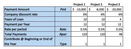
A company is considering investing excess cash into a project. There are 3 project options available, each with differing monthly payment contributions and total payments. The company would like to better understand the present value of future cash flows required to fund each of the projects. Project funding is required at the beginning of each month.

Solution:
We can use the PV formula in Excel to calculate the present value of future cash flows required to fund each of the 3 projects.
Formula Implementations:

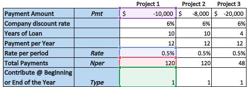
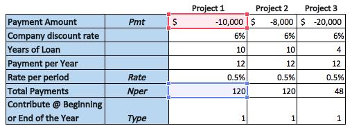
- PV Formula

- Total Payments

Result:
Key Takeaways
- The company can now analyze which options it wants to pursue and it knows that project 2 is going to be the cheapest in terms of the present value of the cash required to fund it.
- Project 3 is in the middle in terms of the amount of money that is required to fund it, while project 1 is the most expensive in terms of the cost to fund it.
I hope that helps. Please leave a comment below with any questions or suggestions. For more in-depth Excel training, checkout our Ultimate Excel Training Course here. Thank you!


0 Comments