

How to use Record Macro Function in Excel to Automate Database Reports?
Automation of Database Reports with the Record Macro Function is useful when you export database reports in excel for your everyday reporting purposes. For example, preparing inventory reports or conducting sales analysis and there is a certain set of repeated steps that you must always follow to prepare the report. If you have identified the steps that are repeated all the time, you can be easily automate them to save time.
In this post, I will explain to you how to use the Record Macro Function in Excel to Automate Database Reports.
Practical applications of Automating Database Reports with Record Macro Function.
Example
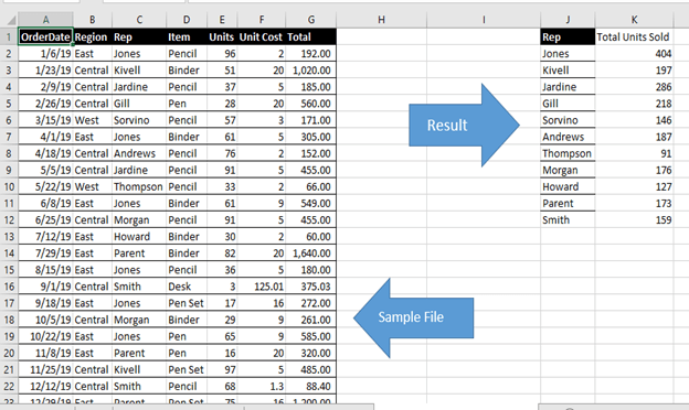
Suppose you have a sales database report and you would like to automate it so that you can calculate the total units sold by each sales representative.
Step 1: Save your Excel file as Macro Enabled Workbook.
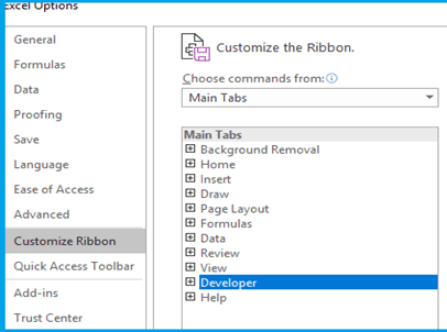
Step 2: Enable Developer Tab in your workbook. Go to File>Options>Customize Ribbon>From Drop Down Select Main Tab>Developer Tab>Add>OK
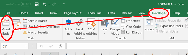
Step 3: From the Developer Tab, click Record Macro and this will prompt you to a Macro Window.
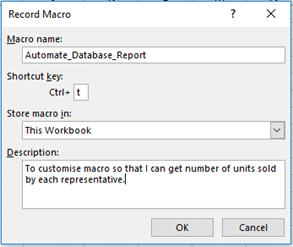
Step 4. (i) Select a name for the Macro. Please note that any spaces in the name should be filled with underscore “_” as it does not allow spaces.
(ii) Select a short cut key (optional).
(iii) Option to store the macro in either the same workbook or elsewhere.
(iv) You can add a description so that you can remember the reason why the macro was created (Recommended).
Step 5: Once you press “OK”, the macro will start recording automatically.
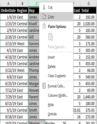
Step 6. You can now proceed to carry out the activity on your database workbook the same way you want it to be automated. In the example above, we will select column C and paste it in Column J. Please make sure not to use any shortcut keys as this can confuse the VBA editor.
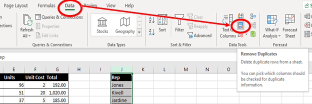
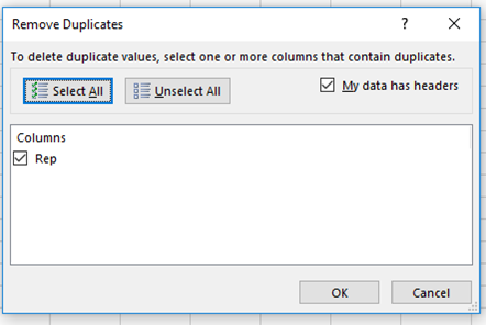
Step 7. Select Column J and go to Data Tab > Remove duplicates. A remove duplicates dialogue box will appear, press OK to get unique representative names.
Step 8: Now Select Cell K1 and name it “Total Units sold”. Below it, type the SUM IF formulae “=SUMIF(C:C,J2,E:E)”. Drag and paste the formulae against all the empty cell. Please make sure not to paste in on the entire column as it will make the worksheet heavy.
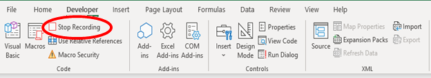
Step 9. Go to Developer Tab>Stop Recording. This will stop recording the macro and save it.
Step 10: To view how the VBA has recorded your macro, go to Developer Tab>Visual basic. This will open the VBA editor showing how the formula has been saved. Check for errors and correct them. The formula should look like provided below.

Explanation of the VBA Code
The VBA code shown above is further explained below for the users to understand so that they can customize it themselves if they want the result to be different as per their needs.
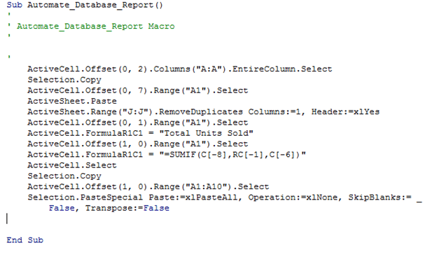
ActiveCell.Offset(0, 2).Columns(“A:A”).EntireColumn.Select
The first layer is simply the Offset function which directs excel to move from one cell to the other based on a specific row and column number. In the beginning, the pre-defined excel cell will be the Cell A1. So, from the Syntax, we are telling excel to move zero rows and two columns forward from the cell A1. Once excel moves to cell C1, we are asking it to select the entire column.
Selection.Copy
The second layer is instructing excel to copy the selected column.
ActiveCell.Offset(0, 7).Range(“A1”).Select
In the third layer, we are again using the offset function. Please note, that in this case, the Active Cell has now changed to C1 because of previous selection. After moving seven columns forward from the cell, the new active cell will be the cell J1.
ActiveSheet.Paste
The fourth layer is instructing excel to paste the copied column on the new active cell.
ActiveSheet.Range(“J:J”).RemoveDuplicates Columns:=1, Header:=xlYes
The fifth layer is the remove duplicates function. We are simply selecting the entire Column J and removing the duplicate values. The Syntax is also defining that the data for remove duplicates is in one column and it contains a header as well.
ActiveCell.Offset(0, 1).Range(“A1”).Select
The sixth layer is simply the offset function to select cell K1.
ActiveCell.FormulaR1C1 = “Total Units Sold”
In seventh layer, we type the header.
ActiveCell.Offset(1, 0).Range(“A1”).Select
In the eight layer, we are instructing excel to move one row downwards.
ActiveCell.FormulaR1C1 = “=SUMIF(C[-8],RC[-1],C[-6])”
In the ninth layer, we can see that now the active cell is K2. The code simply enters the SUM IF formulae where it selects the Column C having the representative names and Column E having the total units sold. The negative numbers represent corresponding column distance from selected cell. Leftward or upward cell movements are represented by a negative sign.
ActiveCell.Select
Selection.Copy
ActiveCell.Offset(1, 0).Range(“A1:A10”).Select
Selection.PasteSpecial Paste:=xlPasteAll, Operation:=xlNone, SkipBlanks:= _ False, Transpose:=False
The Last part of the VBA code is simply copying the SUM IF formulae to the rest of the representative names to give the result next to each representative name.
Now that you understand how the Record Macro works in Microsoft Excel and stores the VBA Code to automate database reports, you can also customize it as per your needs.
I hope that helps. Please leave a comment below with any questions or suggestions. For more in-depth Excel training, checkout our Ultimate Excel Training Course here. Thank you!


0 Comments