How to Use the IPMT Formula in Excel
The IPMT formula returns the interest payment for a given period for an investment based on periodic, constant payments and a constant interest rate.
This is something you can use to calculate investments or also loans and it will return the interest payment for a specific period that you are trying to find. You can also create a loan amortization schedule out of the IMPT formula to help you with it.
Formula:

Formula Explanation
- Rate (required): The interest rate per period
- Per (required): The period number for which you want to find the interest.
- Nper (required): The total number of payment periods in the annuity.
- Pv (required): The present value, or the lump-sum amount that a series of future payments is worth right now. Also, this is the loan amount.
- Fv (optional): The future value or a cash balance after the last payment is made. If fv is omitted, it is assumed to be 0
- Type (optional): The number 0 (zero) or 1 and indicates when payments are due. 0 (zero) for when “at the end of the period” and 1 (one) for “at the beginning of the period”
Example:
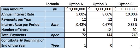
On January 1, 2020, Davidson and Co. acquired equipment through a loan for $1,000,000 payable. The loan has different loan options available (A, B, C below) which vary in interest rate (5% to 10%) and length.

Davidson & Co. would like to know what the interest payment would be in the 12th month of the first year.
Solution:
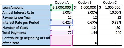
We can use the IPMT formula to determine the amount of interest payment in the 12th month under each loan option.
Formula Implementation:

Result:

- Alternatively, we would create a loan amortization schedule if we wanted to build this out further.
- Now we know how to use Excel to calculate the interest payments using the IPMT formula for a loan or investment.
I hope that helps. Please leave a comment below with any questions or suggestions. For more in-depth Excel training, checkout our Ultimate Excel Training Course here. Thank you!


0 Comments