

How to Use the OFFSET Formula in Excel
The OFFSET formula in Excel is used to return a range that is a specified number of rows and columns from a reference cell or range. This is a unique formula in the sense that it is not often used by a lot of people, and it is particularly helpful in situations where you have a specific template that you need to populate.
It also has a certain order in which it needs to be filled out and the raw data is produced from a source system in a backward fashion or not in the fashion that you need to be in the template that you’re preparing.
Formula
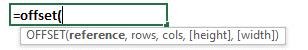
Note that a negative value can be used in the formula. If a negative is used, then instead of having the OFFSET lookup a value below (row) or to the right (column), a negative value will lookup above (row) or to the left (column).
Formula Explanation:
- Reference: The starting point of reference. This is a cell reference.
- Rows: The number of rows to offset below or above (if a negative value is used) the starting reference.
- Cols: The number of columns to offset to the right or left (if a negative value is used) of the starting reference.
- Height: [optional] The height in rows of the returned reference.
- Width: [optional] The width in columns of the returned reference.
Example #1:
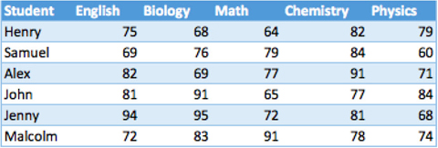
We have a list of grades of students below. The goal is to find:
a) Math grade for John
b) Sum of John’s grades for all subjects.
Solution #1:
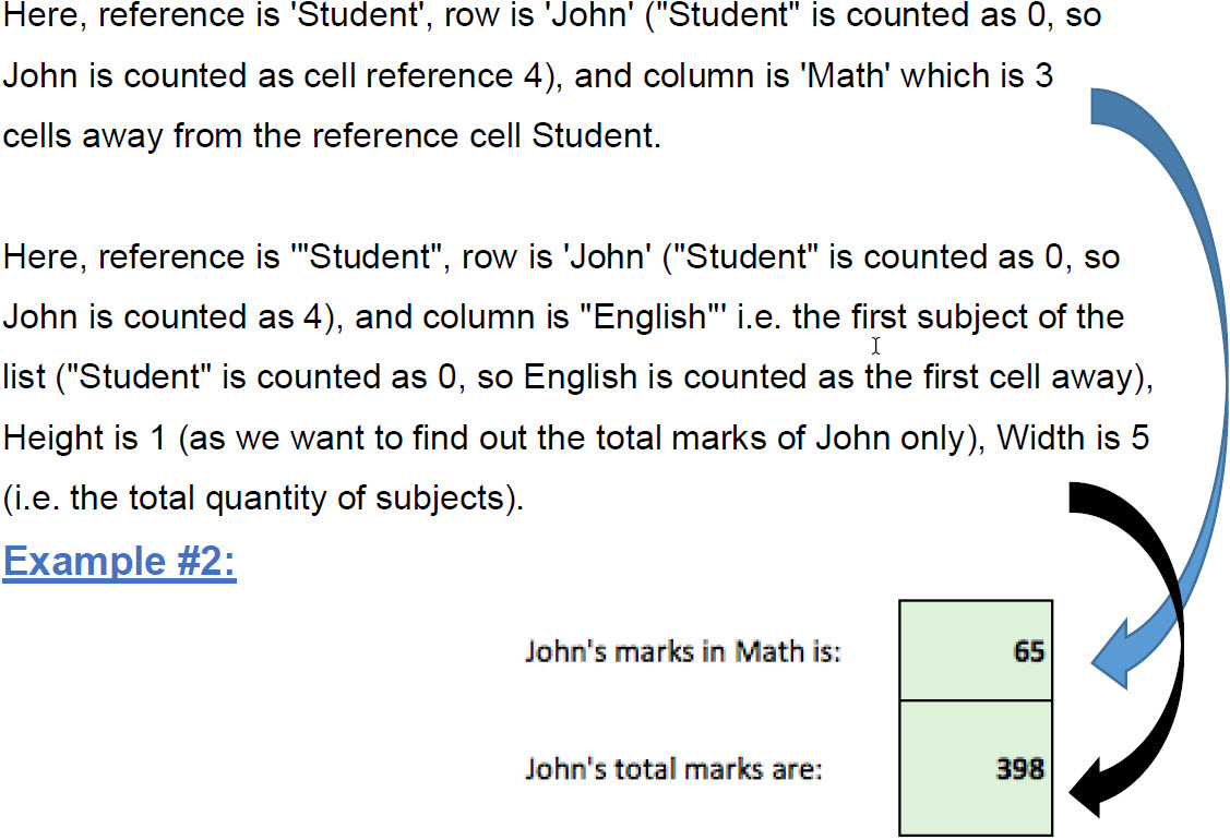
We can use the OFFSET function with the first cell of the table “Student” being our relative reference point for the formula.
The OFFSET function is also convenient when you need to lookup data in a table that has dates that are in a contradictory order to the table you are creating.
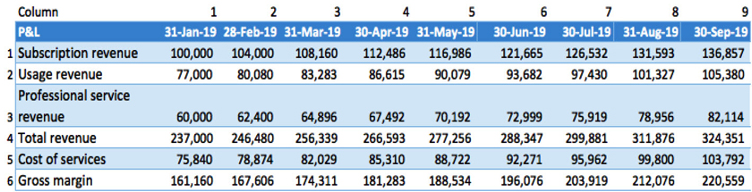
For example, below is the P&L of HBC Inc. The earliest date appears in the left column and the most recent date appears in the right column. Let’s assume we need this data in reverse chronological order.
Solution #2:
In order to reverse the order of the data, we can use the OFFSET function with the P&L header’s first cell to be the reference cell.
For example, for the subscription revenue September 30, 2019 cell, we will reference the first row below P&L and column 9 that comes after the P&L cell.
=OFFSET(C46,1,9) returns the result: $136,856.91
- Taking this a step further, we can automate the formula so that we can drag it throughout the table and have it pull the correct cell reference.
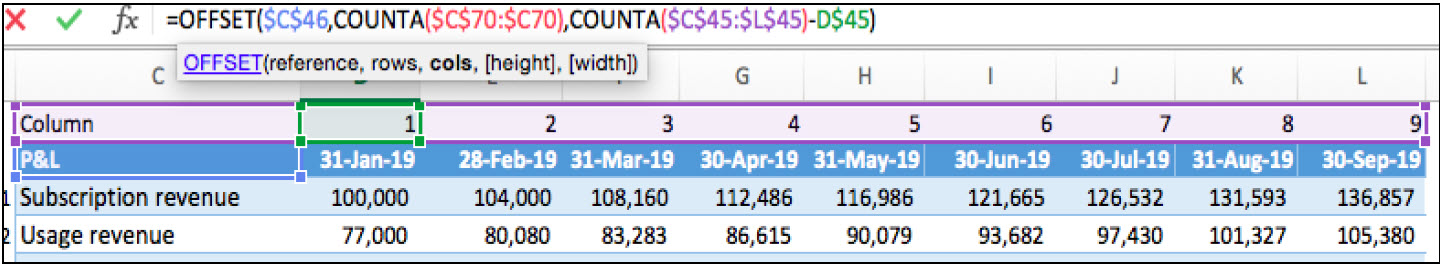
In order to do this, we need the OFFSET formula to calculate the September column as being offset to column reference 9, the August column being offset to column reference 8, etc. This can be achieved by embedding the COUNTA formula in the OFFSET formula and counting the number of columns that exist in the table and subtract the current column reference in the above table. For example, the first month’s column in the above table is 1 and last month is 9. Total column count = 10 including the P&L column.
Therefore, 10-1 = 9 and should be used as the column OFFSET when rearranging the data in the below table. We can take a similar approach for the rows (i.e. subscription revenue being the first-row offset, and gross margin is the sixth row offset.
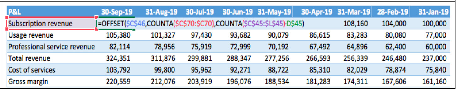
- For the September 30, 2019 column below, we use this formula:
=OFFSET($C$46,COUNTA($C$71:$C71),COUNTA($C$45:$L$45)-D$45)
Formula Implementations:
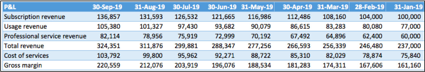
Result:
I hope that helps. Please leave a comment below with any questions or suggestions. For more in-depth Excel training, checkout our Ultimate Excel Training Course here. Thank you!


0 Comments