

How to Create a Pivot Table in Excel
Pivot tables are useful when you have information in a table and you’d like to quickly rearrange the data without the use of a formula based on filters or present it differently.
Pivot tables can provide a flexible analysis. However, it does not automatically refresh and if you modify the source table data it may break.
Steps:
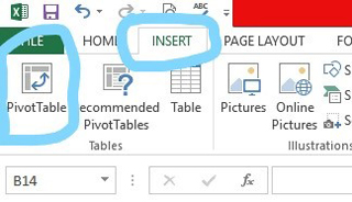
1. Click any blank cell in the worksheet.
2. From the INSERT tab click on the Pivot Table.
3. Then organize the data as you’d like it presented.
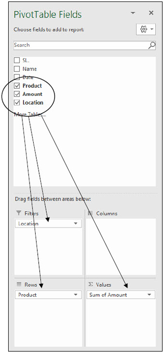
In the Pivot table field list, there are 4 boxes.
- Report filter: Report filter is used to display conveniently a subset of data in a PivotTable report or PivotChart report.
- Row label: Fields put in the row label are listed on the left column of the table.
- Column label: Fields put in the column label have their values listed across the top row of the table.
- Values: Fields put here are summarized and added in the table.
Example:
You are a sales executive of a company named USA Hardware Company. You have a list of sales of some hardware products, and you are required to the amounts sold by-product for the Midwest.
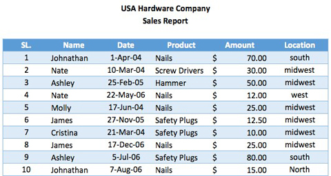
*Note this table is only a sample of an example with few data entries, and the formulas are based on the whole population of raw data which are not reflected in the example.
Solution:
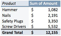
1. We have created the below PivotTable with:
- Report filter = Location set to midwest.
- Row label = product column
- Column label = blank
- Values = amount column
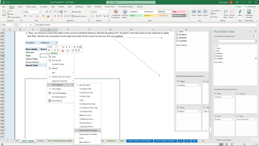
2. Then, we choose to insert the table in the current worksheet (below), click the dropdown for “location” and only check on the midwest to apply that filter. Review the screenshot to the bottom of the screen to see how this was applied.
Screenshot:
Here’s how to arrange the data in the PivotTable and stack rank it:
As you can see, Pivot Tables are quick and easy to be able to slice and dice information and get it the way you want to. I can also rearrange the data within this table by going to Pivot Table Analysis, clicking on Field List, and then modifying the product, amount, and location fields to suit your needs and rearranging the format accordingly.
This is the beauty in using pivot tables, they are very flexible to create quick analysis!
I hope that helps. Please leave a comment below with any questions or suggestions. For more in-depth Excel training, checkout our Ultimate Excel Training Course here. Thank you!


0 Comments