

How to Use the VLOOKUP Formula in Excel
When you have a specific item you’d like to lookup in a table and there is only one of that item in the table i.e. it is unique. This uses a vertical lookup.
Separately, you could use the HLOOKUP formula but the HLOOKUP formula is when you are making a horizontal lookup from a row. This vertical lookup is when you are looking up data within columns
Formula
Formula Explanation:
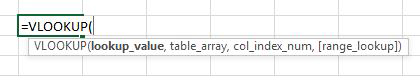
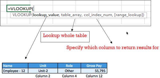
- Lookup value: Cell which you would like to reference and lookup in the table.
- Table array: This is the range/array of data from which we want to lookup our lookup value. Note that the lookup value must be in the left-most part of the table array.
- Col_Index_num: It is the column number from where we want to return the result.
- Range_lookup: This refers to either wanting an exact match or close match.
Example #1:
Employees who work for Home Depot are organized into units and roles. They have employee designation codes depending on their role.
The Financial Analyst needs to be able to obtain information for any particular employee at any time using raw data exported from the company’s HR database. The Analyst would like to perform a lookup of an employee’s unit, designation, and gross, pay.
Solution:
The Analyst uses the VLOOKUP formula to lookup the employee name in the HR database table and returns the result of the unit, designation, and gross pay above.
The Analyst uses the VLOOKUP formula to lookup the employee name in the HR database table and returns the result of the unit, designation, and gross pay above.
Example #2:
Assume the Analyst is working with a very large data set and the columns are occasionally shifted. If you were to insert a column after column C, the above formula break because the unit lookup is to column 2. If we insert a column to the table after the name column, column 2 will be blank. How do we overcome this hurdle so that the formula does not break if columns are inserted?
Solution:
Instead of using the simple VLOOKUP formula, we can use the VLOOKUP formula in combination with the match function so that we perform a MATCH of the headers we want to pull information into the above table (unit, role, and gross pay).
Therefore, our formula looks like this:
Updated formula with MATCH:
=VLOOKUP($C$36,$C$42:$O$481,MATCH(D$35,$C$42:$O$42,0),FALSE)
Old formula without MATCH:
=VLOOKUP(C22,C44:O483,2,0)
- Notice that the only thing that changed was the insertion of the MATCH formula where column “2” was in the old VLOOKUP formula.
The updated table of results with the VLOOKUP MATCH formula is below.
- Now if you try to insert a column in the worksheet after column C, the solution 1 table will break but the solution 2 tables will remain accurate with the results.
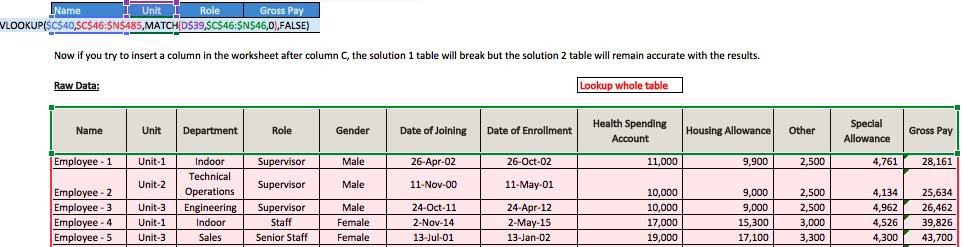
* Note the tables above are only a sample of an example with few data entries, and the formulas are based on the whole population of raw data which are not reflected in the example.
Summary
The VLOOKUP with MATCH Formula is a very handy way of preparing a VLOOKUP formula. It is preferable to use the VLOOKUP or HLOOKUP with an embedded MATCH formula for the reason that it just ensures in the long run if you are going to be doing a lot of financial modeling or analysis, your data will not break, and has more flexibility as you do not have to update the column numbers if anything changes later on.
I hope that helps. Please leave a comment below with any questions or suggestions. For more in-depth Excel training, checkout our Ultimate Excel Training Course here. Thank you!


0 Comments