These 20+ formatting tips will help make things easier on the eye!

Good presentation is crucial for a good impression on top management and provides an easier way to look at your work.

1) How to hide Page Layout/Disable View Gridlines in Excel

Hiding the gridlines is a good way to make the worksheet look more smooth and very easy on the eyes. It can be done by going on “View” and checking on the “Gridlines” button.

The Gridlines provide the usual reader of an Excel Workbook a level of clarity, but it is better suited for presentation purposes to someone who simply wants to review a workbook rather than modifying it.

2) How to use Format Painter in Excel

The Format Paint function can be helpful when you want to copy the formatting of a certain cell and is actually a better alternative to “Copy” and “Paste” since it is faster.

To make a cell the same format as another, click the paint brush button on the top left ribbon.

3) How to Clear Formats in Excel

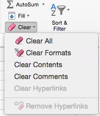
You can Clear formats (font, size, gridlines, etc.) to clarify and cleanse data to its raw format. Click on the “Home” button on the top ribbon, navigate to the “Clear” button on the right side, and then click the “Clear Formats” button.

4) How to Remove Formula Errors in Excel

This key formatting tip is often used when using formulas like the VLOOKUP because if the VLOOKUP function does not return what you’re searching for, then it would result in an error.
By inserting the function “=iferror(),0)” it will show a “0” instead of errors such as #VALUE!, #DIV/0!, etc. making it look less aggressive for someone reviewing your work.

This is also beneficial if you are calculating the sum or using other formulas on a certain set of data. If there are formula errors in that data, you won’t be able to run a formula on it but if the formula errors are removed then it won’t give a formula error when running a summation.

5) How to Insert a 0 at the beginning of a cell in Excel

Use the ‘ to insert a 0 at the beginning of a cell. This is particularly useful since 0’s generally disappear from cells regardless if you put them or not.

In the first row above, the 0 was written without the apostrophe, and then written with it before entering 63 on the second row, hence showing the difference.

6) How to Freeze panes in Excel

You can Freeze panes so that the viewer doesn’t have to guess or scroll back up to the header to view the header’s name or date.

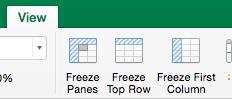
Do this by going on “View” and clicking on “Freeze Panes”. The ‘Freeze Top Row’ function locks up the first row so you can view it as you scroll down back and forth anywhere on the workbook. The ‘Freeze First Column’ function similarly locks up the first column so you can view it while scrolling back and forth, right and left of it anywhere on the workbook. The following are examples the before and after effects of applying Freeze Panes.

Normal View

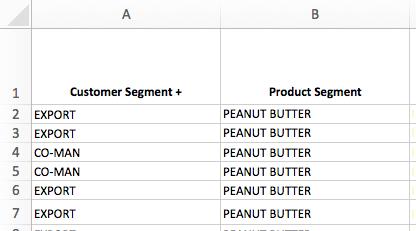
Freeze Panes

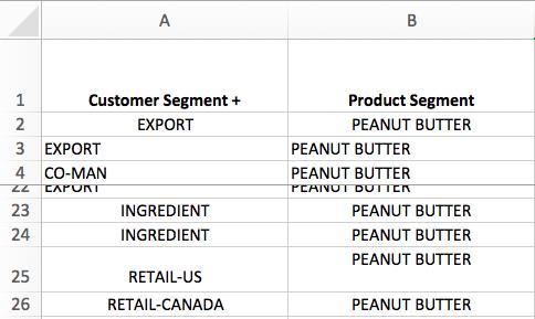
In the example above, the 5th row have been frozen using the ‘Freeze Panes’ option allowing me to scroll up and down, left and right while still having the view of the 4 rows above it.

Freeze Top Row

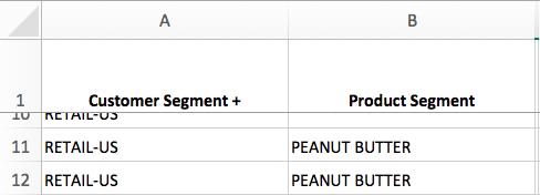
In the case above, the ‘Freeze Top Row’ option was used and it can be seen how it froze the first row while you can scroll down to the 11th and 12th rows and still have the access to it.

Freeze First Column

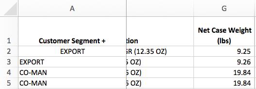
The ‘Freeze First Column’ option was used above and it can be seen how moving left and right does not affect the first column as it always stays fixed as a reference.

6) How to change Date Formats in Excel

It is important that you choose a date format and be consistent with it throughout a financial model. The following image illustrate the short date and long date format options.

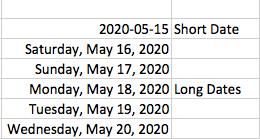
Click on date cells and format cells as dates and make a selection between the short and long date formats as shown above.
The following are the different date format options in Excel. These allow users to select a date format that best fit their needs.

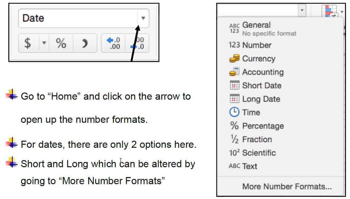
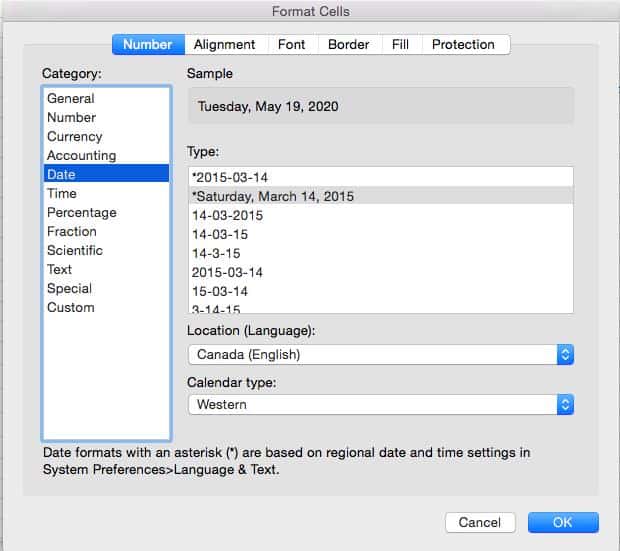
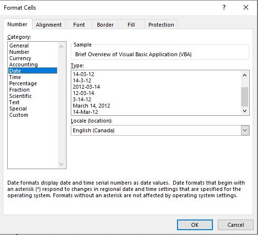
• The “More Number Formats” open up the Format Cells options that list the categories for different versions of dates.
• All of the formats can be selected from here, but the most professional version is on the bottom picture in the standard format of March 14, 2012.
• However, different places require different formats so it is preferential.
• The Format Cells also features alignment, font, border, and color fill, all of which are used for financial statements such as P&L. The benefits of these features will be discussed later in the blog

8) How to Lock Cells in Excel (Tip – Click F2 to enter cell)

Locking Cells is a good way to maintain consistency when applying formulas.

You can lock cells to avoid movement when copying formula to another cell by applying the ‘$’ before the rows and columns you want locked. ‘$’ sign before the row locks the row cell, and the ‘$’ sign before the column number locks the column.

9) How to use Home/word wrap in Excel

The Word wrap text tool in Excel allows you to consolidate texts within a cell and avoid it going into the subsequent cells. Simply go “Home” and highlight the desired column, shifting the width of the desired column, and then clicking the “Wrap Text” button.

10) How to Use Review Spelling in Excel

Making spelling mistakes in any profession seems unprofessional. The spelling option in Excel is a proofreading tool that reviews for any mistakes and is the perfect tool when writing technical reports, essays, research, etc.

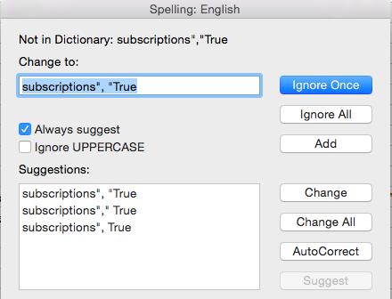
Simply go to the “Review” section and click on “Spelling” to check for any spelling errors. Once it opens, you can decide to ignore the word(s) and/or even change it to a suggested word from the ‘Suggestions’ box.

11) Why and How to Use “Align” in Excel

The Alignment tool in Excel is an effective way to indent cells without affecting their values or formulas. You can present subtotal data properly without inserting spaces so that formula can still be used on the cells. This can be done using the align signs for left and right from the “Alignment” section from the “Home” tab.

The following entries show the difference between the effects of an alignment change when compared to adding spaces. The first 2 formulas entered were to give the result ‘true’ if the words ‘’subscriptions’’ and “usage” matched with the text written in the quotation of each formula after the ‘=’ sign. The F43 refers to the cell in green, while F44 refers to the cell in blue. When there no changes being made, the results equate to being ‘true’ as the words clearly match.

However, when we make changes in formatting using alignment using spaces, we see different result. The aligned “subscriptions” cell above in grey remains true as we used the alignment function in Excel to push the text to the right.

On the other hand, in the brown cell above for “usage” there were manual spaces added before the word “usage.” This changes the text in the cell and therefore when we run formula on the cell to lookup the word “usage” it cannot find that word in the cell and the result is false.
Therefore, it is a better idea to use the alignment function in Excel as opposed to using manual spacing.

12) How to Highlight Data Table in Excel

When you have a long list of client emails and need to write their names beside it, this Excel tool will help you solve this problem. In order to highlight the data table, click “Control + E”. The purpose of a flash filling is that it will automatically infer the first and last names from a list of emails if presented by that order.

14) How to Set up a P&L for Presentation?

When it comes to setting up financial models, it is important to make it look neat, organized, and professional. The following model is an example of a P&L setup with the inclusions of borders, italics, and modified rows and columns.

This format divides up the actual and forecasting data for revenue through 2020 for all 4 quarters.
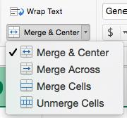
For example, you can make the top header have a color fill and use white text. You can also implement a border using the border function and choose any color, for example black. Lastly, you can also merge cells for cases like the actual and forecast section using the “Merge” button on “Home”.

15) Using the Instructions Tab in Excel

If you’re preparing a financial model, it would be beneficial to implement an instructions tab in Excel dedicated with instructions on how to update the financial model. This will allow others who open the file for review or entry to have a guideline on how to operate the workbook catered to your style.

16) Using the Assumptions Tab in Excel

Following on that, the assumptions Tab is another fundamental aspect to add to the P&L to make it more detailed and informative for the viewer as it would have a tab dedicated with key assumptions built into the financial model and make use of the variables.
If you are building a financial model, it is worthwhile to have an assumption Tab as when you make changes to it, and when it gets modified, it would update the rest of the workbook. You should set it up so that the assumptions can be modified on the assumptions tab which would allow you to do this.

17) How to Summarize Data in Excel

Place the data along with the columns and summarize data into fiscal quarters and years. This is one of the best ways to organize data as it is similar to the way financial statements are prepared. Moreover, another key aspect is placing the most recent data on the right side as most people tend to read from left to right. Hence, it is best to start with the oldest data on the left side and more recent on the right side.

18) How to Highlight Cells in Excel

It’s a best practice to have standardized formats for the meaning of cells so it is well understood by the user.

It is important to limit the number of highlights you use. If you do use highlighting, make sure that you have a legend in your workbook that indicates what all the highlights mean.
Furthermore, if you are building a financial model consider having all input cells/ variables filled with a specific color, for example, blue. That way the user will know that if they change the contents of a cell that is blue, it will vary the results of the financial model because it is an input cell and it has dependencies.

You can also use the yellow highlight to indicate cells that have issues or requires further investigation, or red as another example. And then all the other cells can be given another color, in this case, a clear background.

Overall, it is important to have some sort of a legend that notifies the reader of its significance and offers a clear guide as to what each color represents. It also directs people as to what colors to use when contributing to that specific workbook which ultimately creates a better flow in terms of clarity and presentation.

I hope that helps. Please leave a comment below with any questions or suggestions. For more in-depth Excel training, checkout our Ultimate Excel Training Course here. Thank you!