What is Conditional Formatting in Microsoft Excel? How is Conditional formatting used in a project?

Conditional formatting in Excel enables you to highlight cells with a certain color depending on the cell’s value. This is a beneficial function when you want to draw attention to data that meets certain value criteria.

In this post I will explain you how to use conditional formatting function can be explained with the help of following example:

Practical applications of Conditional formatting function

Example 1

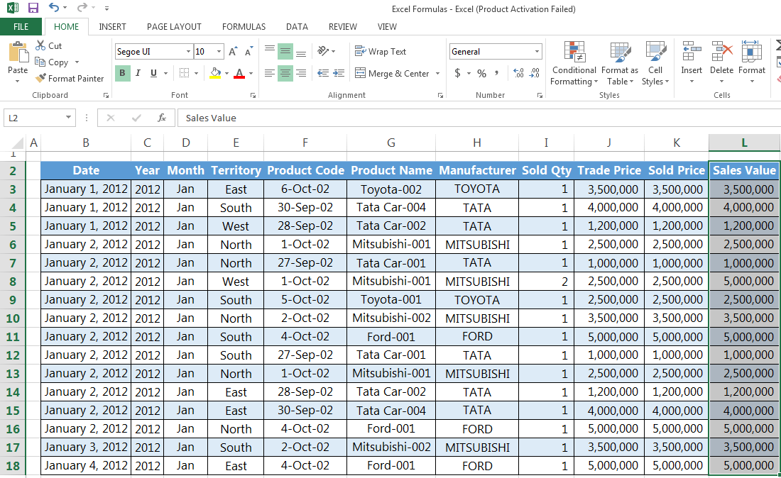
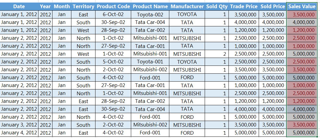
Suppose you have a sales report for January 2017, and would like to highlight the sales that are less than 4,000,000.

Step 1: Select the row or column that you want to format

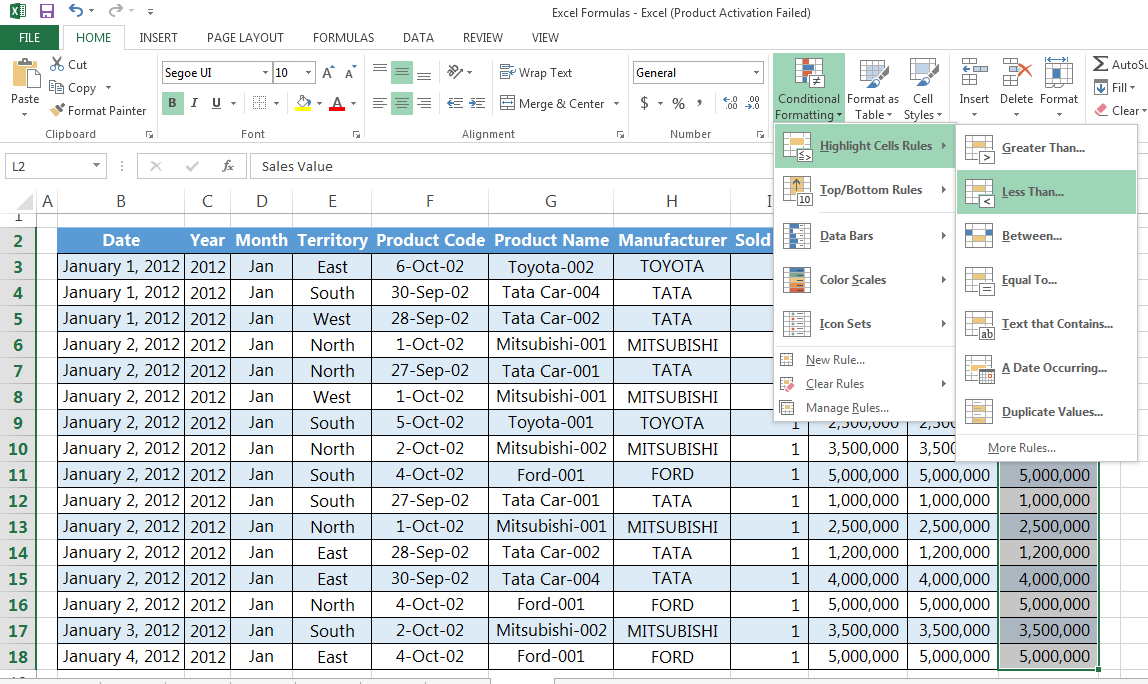
Step 2: Go to Home tab > Conditional formatting > Highlight cells rules > Less than

Step 3: Insert value on format cell that are LESS THAN, and set your condition (e.g. Light Red Fill with Dark Red Text

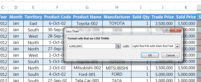
Step 4: Then click OK

Example 2

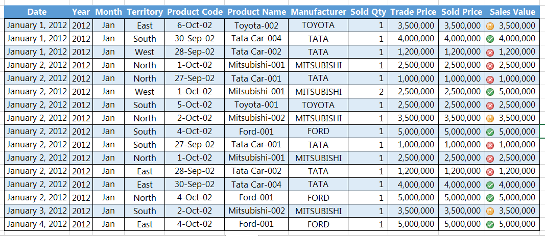
Suppose you have a sales report for January 2017 and would like to indicate beside the sales values certain symbols depending on whether they are at satisfactory level or not based on the following conditions:

• >$4,000,000, denote with checkmark sign,
• <$4,000,000 and >$3,000,000, denote with an exclamation mark sign,
• <$3,000,000 denote with a cross mark

Step 1: Select the row or column that you want to format

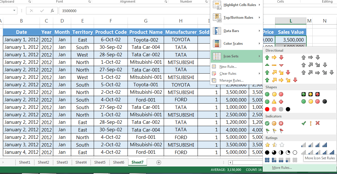
Step 2: Go to Home tab > Conditional formatting > Icon sets > More rules

Step 4: Modify the rule based on your preferences. In our example, we have selected the respected signs as were required in the report and have giving the numeric conditions accordingly

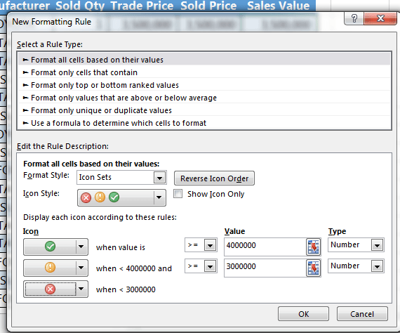
Step 5: After selecting the required signs and mentioning the numeric conditions, click OK

I hope that helps. Please leave a comment below with any questions or suggestions. Thank you!