How to Use the HLOOKUP Formula in Excel

The HLOOKUP formula in Excel is used when you have a specific item you’d like to lookup in a table and there is only one of that item in the table i.e. it is unique and you want to reference something that exists within a row.

This is in contrast with the VLOOKUP formula where you are looking up something within a specific column and you are trying to count over to the right side. Whereas, HLOOKUP is looking up horizontally, not vertically.

Formula Explanation:

• Lookup value: Cell which you would like to reference and lookup in the table.
• Table array: It means the set of data from which we want to lookup our lookup value.
• row_Index_num: It is the row number from where we want to return the result.
• Range_lookup: This refers to either wanting an exact match or close match.

Example #1:

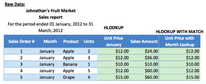
You are a Sales Executive of a company named Fresh Market. You have a list of product sales in a sales report spreadsheet but the report only shows the quantity of sales and not the unit price or sales dollar amount sold.

The unit price is in a separate table and you want to be able to pull it into the sales report table and show the unit price and sales dollar amount alongside the rest of the data in the sales report.

Solution:

Using the HLOOKUP function, we can perform a lookup of the product type (e.g. apple) to the second table which shows the unit price information.

Once that information is pulled into the report, we can multiply unit sales by unit price to determine the total sales amount.
           i.e. price x quantity = revenue

Example #2:

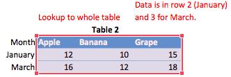
Assume you are working with a very large data set and the rows are occasionally shifted. If you were to insert a row in table 2 below between the first and second row, the formula would break because the lookup is to row 2.

If we insert a row to the table after the header row, the second row will be blank and we are referencing row 2 of the table in our HLOOKUP formula. How do we overcome this hurdle so that the formula does not break if rows are inserted?

Also, example 1 assumed the pricing was static throughout the year. What if the pricing increased in March for each of the products?

Solution:

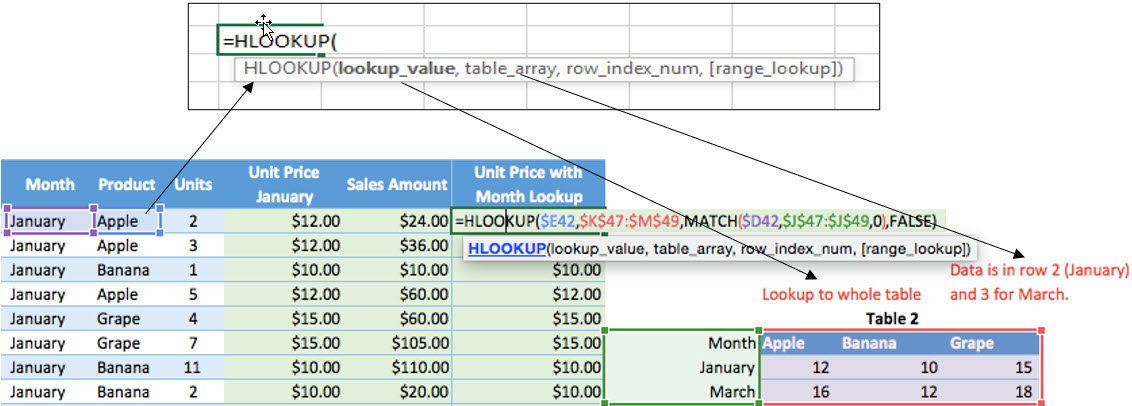
Instead of using the simple HLOOKUP formula, we can use the HLOOKUP formula in combination with the MATCH function so that we perform a match of the headers we want to pull information into the table based on the product description.

We can also match the month to the date in the table so that we are pulling in the correct pricing based on the date of the sale. Therefore, our formula looks like this:

• Updated formula with MATCH:
  =HLOOKUP(E42,J47:L49,MATCH(D42,$I$47:$I$49,0),FALSE)
• Old formula without MATCH:
  =HLOOKUP(E45,HLOOKUP!$J$50:$L$51,2,0)

Notice that the only thing that changed was the insertion of the MATCH formula where row “2” was in the old HLOOKUP formula.

Formula Implementation: HLOOKUP

Reference Table

Formula Implementation: Sales Amount

Formula Implementation: HLOOKUP with MATCH

Result:

* Note the tables above are only a sample of an example with few data entries, and the formulas are based on the whole population of raw data which are not reflected in the example.

Summary

The HLOOKUP with Match formula is a second way in which you could use the HLOOKUP formula with an embedded MATCH formula.

It is a preferred method due to the versatility it provides and if you were to ever insert a row or move around data within your data table that you are performing to look upon, you would not have to worry about things getting messed up when you move around the data.

I hope that helps. Please leave a comment below with any questions or suggestions. For more in-depth Excel training, checkout our Ultimate Excel Training Course here. Thank you!