

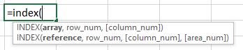
How to Use the INDEX Formula in Excel
The Index formula is typically used to return the value of an item in a table depending on the row and column number chosen to be indexed in the formula.
The Array Formula Syntax Includes:
- Array (required):- This is a range of cells.
– If the array contains only one row or column, the corresponding row_num or column_num argument is optional.
– If array has more than one row and more than one column, and only row_num or column_num is used, INDEX returns an array of the entire row or column in array.
- row_num (required) – This selects the row in the array from which to return a value. If row_num is omitted, column_num is required.
- column_num (optional) – This selects the column in the array from which to return a value. If column_num is omitted, row_num is required.
Example Using the INDEX Formula In Excel:
The General Manager of a second-hand car dealership wants to know the quarterly sales of each branch for a particular quarter and wants to be able to look it up with ease.
The Financial Analyst generates the Sales Report of the dealership’s sales for the current year per below.
However, the General Manager doesn’t want to have to constantly sort through data. The General Manager wants a picklist to be able to choose which quarter he would like to pull data from with corresponding data for the branch location and vehicle type.
The Financial Analyst is able to reference the quarterly sales by state using the INDEX function and create 3 picklists (Quarter, Branch Location, Type of Vehicle) to create this financial model for the General Manager.
Solution:
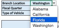
In our solution, we created a drop-down menu for the General Manager so that they would have the ability to quickly toggle between options and determine the result.
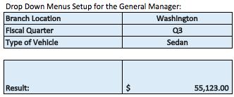
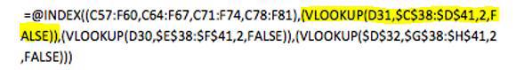
The “Result” field using the INDEX formula to perform a lookup of the sales data based on the parameters selected (Sedan sales during Q3 in Washington). Below is the formula written for the INDEX formula located in the “Result” cell.
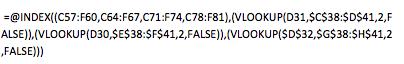
In the above INDEX formula, sales data is being indexed based on criteria including fiscal quarter, branch, and vehicle type. The VLOOKUP formulas are looking up the data in the below table which we created to help lookup data within the array tables of the raw data.
In order to create the drop-down menu setup for the General Manager it was a two-step process:
1. Create an index formula based on the above tables.
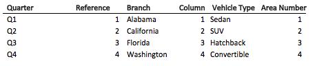
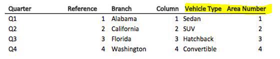
2. Create picklists that perform VLOOKUPS against a reference table above which specifies the location of the data within the array table. i.e. Quarter 1 is the first row in the above table, Alabama is the first branch location, Sedans are the first area location.
If we take a look at the formula syntax for the INDEX function, it is comprised of a few components.
I. Array
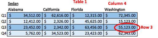
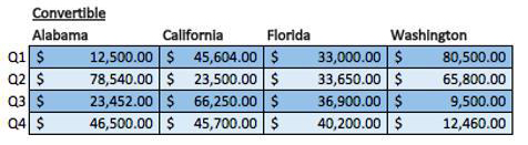
First, we have the array and we already put in the array within the formula which are four tables that exist for the different vehicle types. Below is what the array tables look like for the sales report. There are 4 of these in the sales report (one for SUV’s, hatchback, convertible, sedan) and are each selected as part of the formula
II. Row_num
The row number is the middle part of the formula and the row number that we want to be selected. The arrays start from Q1 and then end at Q4 going in sequence from 1, 2, 3, 4. If we do a VLOOKUP of Q1 as the fiscal quarter, that suggests it is going to be row number 1 of the array. Hence if we changed it to Q2, then that would return the second row of the array.
III. Column_num
The next part of the INDEX formula is to return a column number of which column we want to return the result for in the array table.
We will use a VLOOKUP for this as well to identify the column number, specifically for branch location. This will work because each of the states as branch locations are sequentially ordered from 1 through 4 in the array table. For instance, the first column of the array is related to Alabama, second column is related to California, third is related to Florida, and fourth is related to Washington, showing that it is consistent across each of the tables.
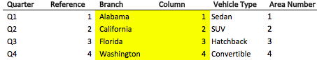
Therefore, if California is selected in the drop-down, then we want to reference column 2. Likewise, if Florida is selected in the drop-down, then we start to reference the third column. As you can see, we are trying to understand the intersection of the row and column based on the drop-down.
I. Reference
In summary, the INDEX formula is applied as follows for our example:
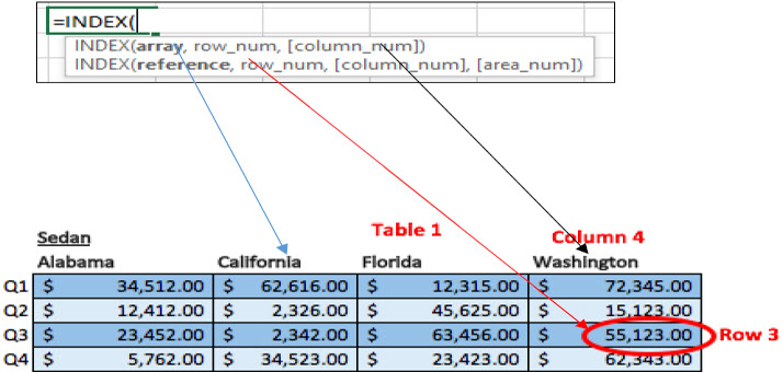
Looking at the fourth column for Washington, the intersection we have highlighted is Washington and Q3 which would be row 3 and column 4 and would return a result of $55,123.
The fourth and final part of the array formula is to reference an area number. We are going to be doing a VLOOKUP for this as well, and the reason why the area number appears is that we referenced four unique arrays at the beginning of the index formula.
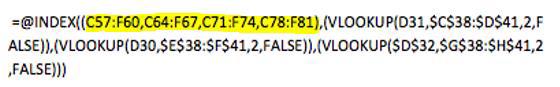
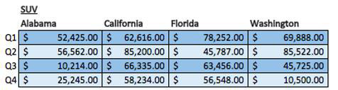
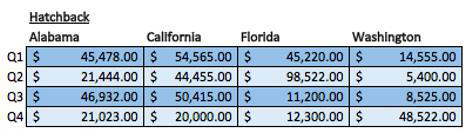
If you recall, we referenced the array for Sedan and then we referenced an array for SUV, then for Hatchback and Convertible. Since there are 4 different arrays, we have to tell the formula which one to reference. We use a VLOOKUP in the INDEX formula to reference our table, find the appropriate vehicle selected in the drop-down, and then accordingly select the area number
I hope that helps. Please leave a comment below with any questions or suggestions. For more in-depth Excel training, checkout our Ultimate Excel Training Course here. Thank you!


0 Comments