The following tips are a MUST for easier navigation in Excel and could you save you a lot of time

How to Toggle Between Excel Files

You can toggle between open Excel files using the Control + Tab key.

It is typically used as a faster method to alter tabs and to switch back and forth with other Excel files. Toggling between Excel files can be a hassle doing it manually, and this shortcut makes it very convenient.

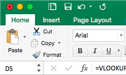
How to Copy, Cut, and Paste Cells in Excel

Copy is used if you want to copy the contents of one cell to another location keeping the original contents of the first location. Cut is used if you want to move the contents of a cell to another location and have it deleted from the previous location. It can be typically used to move formula.

Here are the Shortcuts to Copy, Cut, Paste cells in Excel

• You can copy cells using the “Control + C” key on your keyboard.
• You can paste values that are copied by using the “Control + V” key.
• You can cut cells by using “Control + X” key.

Top Navigation Tips And Shortcuts for Highlighting Data

To save time and work efficiently, these main shortcuts are essential for navigating data within a worksheet in Excel:

• The Control + Arrow keys can be used to move up, down, left, and right within cells. It is used to quickly move between cells within the worksheet.
• The Control + Shift Arrow keys are used to highlight rows and columns depending on the sign of the arrows. Alternatively, the Control + Back shortcut is the best way to navigate back to the top without removing the highlighted selection.
• The Control + A key shortcut is used to highlight all of the data within the table. Further, the Control + A key (hit twice) is used as a shortcut to highlight the entire workbook.
• The Shift + Space bar is used to highlight a row within a worksheet, while the Control + Space bar is used to highlight a column within a worksheet.
• To navigate to the end of the worksheet, the shortcut is Control + End. To navigate back to the top of the workbook and at the start of the worksheet, the shortcut used is Control + Home key.

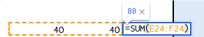
How to Use the Auto-Sum Adjacent Rows/Columns in Excel

You can use the Auto-Sum Adjacent rows/columns to sum for both the values to the left and the values of the top. Simply enter the “Alt +=” key shortcut to auto-sum your adjacent rows and columns.

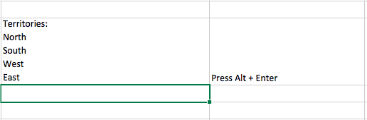
How to Create Multiple Rows In A Cell in Excel

Select within the cell, click the “Alt + Enter” key to create multiple rows in a cell.

It is typically used as a better way to organize data and information, and have multiple sentences or points within a single cell.

How to Insert, Delete, Hide, Move Columns in Excel

The quickest way to insert a column on Excel is by highlighting a row below where you like to insert the new row using the Control + Space bar.

• Then press Control + Shift = to insert a column.
• Similarly, to delete a row, highlight it and press the Control + – button.
• The Control + 0 shortcut is used to hiding a row.
• To identify if there are any hidden rows in a worksheet, simply press and hold the Alt + ; button to highlight the hidden rows and columns in the sheet.
• To undo this action, press “Control + Z”.
• To move a row, simply highlight it by using the Control + Space bar key, hover to the edge of the row, and then click/hold/drag it wherever in the sheet.
• By holding the Shift key, the row will then move locations and shift the other row that was previously there beside it (moves the other column to the right). The purpose is to not delete or override any data in the worksheet.

How to Insert, Delete, Hide, Move Rows in Excel

The quickest way to insert a row on Excel is by highlighting a row below where you like to insert the new row using the “Shift + Space” bar.

• Then press “Control + Shift =” to insert a row.
• Similarly, to delete a row, highlight it and press the Control + – button.
• The “Control + 9” key is used to hiding a row.
• To identify if there are any hidden rows in a worksheet, simply press and hold the “Alt + ;” button to highlight the hidden rows and columns in the sheet.
• To undo this action, press “Control + Z”.
• To move a row, simply highlight it by using the Shift + Space bar key, hover to the edge of the row, and then click/hold/drag it wherever in the sheet. The row will then move locations and shift the other row that was previously there below it.

How to Insert a Datestamp And Timestamp in Excel

The Control + ; key shortcut can be used to insert a Datestamp into a spreadsheet

The ” Control + Shift ; ” is used to insert a Timestamp in a spreadsheet.

This saves you time from having to manually enter a date into a cell in Microsoft Excel. Instead, using the Datestamp and Timestamp shortcut in Excel will save you time if you are often having to input dates into your spreadsheet.

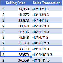
What is the Shortcut to Show Formulas in Excel?

The Control + ‘ key can be used to toggle a view between formula and non-formula view mode. It is typically used when writing formula and can be useful for auditing data, determining how the formula was written, and understanding where the numbers are coming from.

Another way is to go on a cell and hit “F2”, it will open up the formula associated with that cell.

How to Quick Save in Excel

The “Control + S” key can be used to save a file on Excel.

The ‘Quick Save’ options can be used as a shortcut instead of going to ‘File’ and selecting ‘Save’ which takes up a few seconds.

How to apply the Quick Undo Shortcut in Excel

The Control + Z button can be used as a shortcut to undo the previous action on Excel. It is typically used as a quicker method to undo actions rather than going to the top navigation bar and clicking the undo button.

How to Turn Off & On Formula Calculations in Excel

The manual calculation option can be used in Excel for workbooks with large data that lag each time.

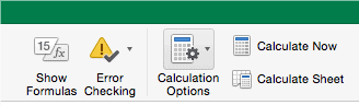
Going to the “Formula” section in Excel, then clicking “Calculation” options and then selecting the manual mode.

Press “F9” to recalculate the workbook to save time having to wait on the workbook to recalculate, update and refresh the numbers.

How to Hide Excel Sheets & Make it ‘Very Hidden’

To make a sheet very hidden instead of just hidden, press and hold “Alt + F11” to open up VBA, then click on the sheet you want to be hidden on the “Properties” section, and then on the ‘Visible’ section on VBA change the dropdown to “Very Hidden”.

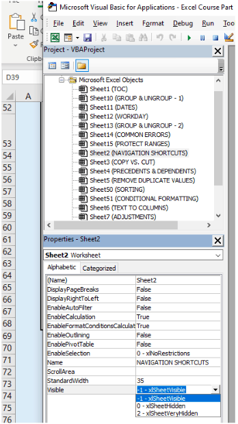
As shown in the ‘Visible’ section for Properties, there are 3 options:

1. Sheet Visible: The sheets appear on the tabs in the worksheet.
2. Sheet Hidden: The sheet will still appear on the list of tabs when you right-click on a tab.
3. Sheet Very Hidden: The sheet will not appear on a hidden tab and disappears completely. To bring it back, open up VBA again and change it to “SheetVisible”.

How to Change Window Size in Excel

If you have multiple files open and you want to do a side by side comparison between worksheets and/or documents, you may need to shrink the size of the workbook’s view.

You can modify the size of the active workbook and its window by pressing and holding the ‘Windows’ key followed by the ‘up’, ‘down’, ‘left’, and ‘right’ buttons.

• Windows key + Up: This changes the window to full-screen mode.
• Windows key + Down: This changes the window to shrink in size.
  *If done twice, it will minimize the file.
• Windows key + Left: Justify the window to the left in a half screen view.
• Windows key + Right: Justify the window to the right in a half screen view.

How to Open Duplicate Window in Excel

Opening up a duplicate window gives you the ability to make a comparison between 2 different areas of a workbook and navigate them both simultaneously.

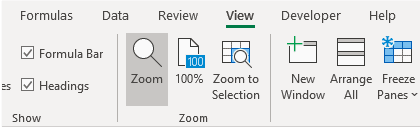
To do this, simply navigate to the ‘View’ tab on the top ribbon, and click on the “New Window” button which will open up the new/duplicate window. Make sure you close that second window and then save the workbook once you are finished working on it to avoid both windows from reappearing.

How to use Formatting in Excel for Texts

The most common ways to format texts in Excel is to use the Bold, Underline, and Italics functions or to change the font color, text style, or text size.

A few common shortcuts which are easy to remember related to Bold, Underline, and Italics and they are the most common for formatting texts.

• To bold a text in Excel: Press “Control + B” on the selected cell.
• To underline a text: Press “Control + U” on the selected cell.
• To italicize a text on Excel: Press “Control + I” on the selected cell.

How to Format Cells in Excel

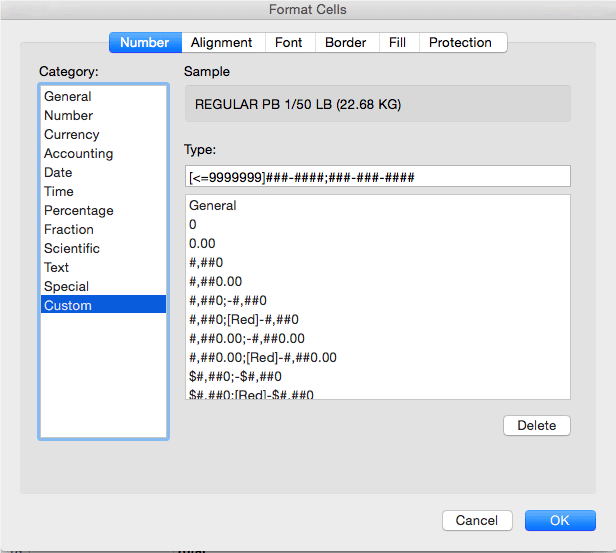
The shortcut to opening up formatting options in Excel is “Control + 1”.

For example, if we change the dollar sign to 2 decimal places, we would change the category to the number and change the decimals to 2 places. This is an effective formatting option for cells because it shows all the categories to format numbers, alignment, font, border, and fills.

How to use the Copy Cell Above Shortcut in Excel 

A quick shortcut to copy down the shortcuts to the above cell in Excel is to click on the cell under it, and then hold “Control + D”.

This will copy down the contents of the cell instead of having to copy and paste the data from above it.

How to Find Keywords in Excel

If you want to do a quick search for a keyword in Excel, press “Control + F” and then simply search the keyword in the dialog box and click ‘Find’.

You can search in either the tabs within the worksheet or the entire workbook by clicking on the search option.

How to Navigate through Excel Sheet Tabs

There are multiple ways to navigate the tabs throughout an Excel workbook.

• To navigate quickly, the first option is by right-clicking on the section at the bottom of the screen where it shows arrows beside the tabs. This will show a pop up a list of tasks to navigate through.

• The second option is to press “F6” and then using the arrow keys to navigate left or right on tabs.

• The third option is by using the “Control + PageUp” (to navigate to the left tabs) and “Control + Page Down” (to navigate to the right tabs) functions. This toggles you through the different tabs of the workbook one at a time.

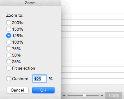
How to Modify Multiple Tab Zoom Levels in Excel

For presentation purposes, it is visually pleasing to keep the same zoom levels for each tab on the worksheet in Excel.

To achieve this, simply go the first worksheet and hold the Shift button, then scroll over to the last tab of the workbook and click on it. Finally, modify the zoom level on the bottom right corner for the selected worksheets.

How to Navigate To A Specific Cell in Excel

The Active Cell Reference function is used to navigate to a specific cell location in an Excel Spreadsheet and can be found in the top left corner beside the formula bar.

This quick function comes in handy when jumping between different areas of a worksheet. The purpose of this function is that it more efficient for large amounts of data.

How to Easily Show Desktop from Excel

• When you have multiple tabs open and want to navigate to your desktop to find a file, instead of clicking on the “Show Desktop” button, you can simply use the “Windows key + D”.
• To switch back to your last active window, repeat the action by pressing and holding the “Windows key + D”

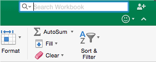
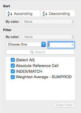
How to Add & Remove Filters in Excel

Filters in Excel are a great way for you to analyze data by viewing specific rows in an Excel spreadsheet while hiding other rows.

• Press “Control + Shift + L” to add a filter in your data set.
• Once you have your data sets with filters ON, you can click on the ‘Filter’ button on the top row and you’ll be able to filter in for example product name, id, #, etc.
• Then if you click “Control + Shift + L” again, it will remove the filter and the data set appears unfiltered again.

I hope that helps. Please leave a comment below with any questions or suggestions. For more in-depth Excel training, checkout our Ultimate Excel Training Course here. Thank you!