How to use the SUM OF BOTTOM N VALUES Formula in Excel

This formula is used to calculate the sum of the smallest or largest set of numbers in an array. The N can represent a specific number of values that you want to calculate. So we are calculating the sum of the smallest subset of data within the array. The bottom number of values within a set of data.

Formula explanation:

Syntax: =SUM(SMALL(array,{1,2,n})) or

SUMPRODUCT(SMALL(array,{1,2,n})) –> both of these formula achieve the same result.
     =SUM(LARGE(array,{1,2,n})) or

SUMPRODUCT(LARGE(array,{1,2,n})) –> both of these formula achieve the same result.

In the above syntax the formulas and arguments refer:

• 1,2,n: The chronological order of a particulars number of values you’d like to calculate the summation of.
• Array: The set of values from which we want to find out the SUM.
• SMALL: Find the smallest values from the array.
• LARGE: Find the largest values from the array.
• SUM or SUMPRODUCT: make the total of selected orders of values.

Example

We have a set of values in the below table containing daily sales. We would like to find out the sum of the smallest 5 sales for the month.

Solution:

SUM of 5 bottom values:

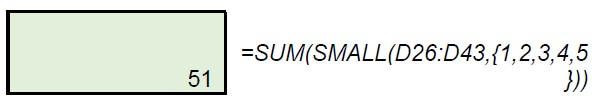
Using the SUM formula nested with the SMALL formula we can calculate the sum of the smallest 5 sales quantities for January 2020.

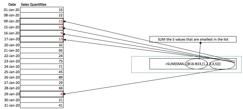
Here, we have determined the sum i.e. 51 of 5 bottom values i.e. 8,9,10,11, and 13.

I hope that helps. Please leave a comment below with any questions or suggestions. For more in-depth Excel training, checkout our Ultimate Excel Training Course here. Thank you!