How to Use the SUMIFS Formula in Excel

The SUMIFS Formula is used to add the numbers which apply when multiple criteria are met. This is different from the SUMIF formula which only relies on one criterion.

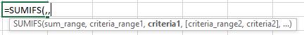
SUMIFS Formula Explanation

     =SUMIFS(sum_range, criteria_range, criteria1, [criteria_range2, criteria2], …)

• Sum_range (required) – This is the range of cells that contain the numerical values to be added together.
• Criteria_range1 (required) – The range that is tested using Criteria1. Criteria_range1 and Criteria1 are considered a pair (criteria1 searches within criteria_range1). Once items in the range are found, their corresponding values in Sum_range are added.
• Criteria1 (required) – The criteria that determine which cells in Criteria_range1 will be added up.
• Criteria_range2, criteria2, … (optional) – This refers to additional ranges and their related criteria. You can enter up to 127 range/criteria pairs.

Example Using the SUMIFS Formula

The General Manager of a second-hand car dealership wants to know how much sales were made during the year for certain cars within certain branch locations.

The Financial Analyst generates a Sales Journal (below) containing the raw data of car sales with product code, product descriptions, and dealer branch location.

Sales Journal:

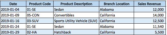
*Note this table is only a sample of an example with 5 data entries while the rest of the data has been cut out for display purposes.

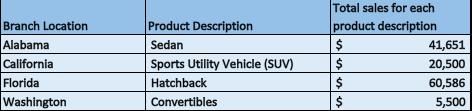
The Financial Analyst can use the SUMIFS formula to summarize revenue by branch and product description for the General Manager in the table below. The “total sales for each product description” column was calculated by using the SUMIFS formula.

To calculate the total sales by a branch location and product description, the formula is syntax is applied as follows:

I. Sum_range formula was used for determining the branch’s sales revenue.

II. Criteria_range1 formula was used for determining the data range of a specific branch location.

III. Criteria1 formula was used for determining a specific branch location.

IV. Criteria_range2 formula was used for determining the data range of what type of product description should be summed in a specified branch location.

V. Criteria2 formula was used for filtering the specified product description.

You can have multiple conditions of criteria which exceed two items, as long as that data is contained within your data table. In this case, we could have extended it further to include a date or product code but in our example, we were only looking for criteria that met branch location and product description.

I hope that helps. Please leave a comment below with any questions or suggestions. For more in-depth Excel training, checkout our Ultimate Excel Training Course here. Thank you!