How to Use the Transpose Formula in Excel

The transpose formula in Excel is used if you are working with data that is either vertical or horizontal and you want to flip it in the opposite direction and present it in the opposite way.

The transpose formula is an array, and this syntax is used to reference data that is to be transposed.

Formula Explanation

ARRAY: This syntax is used to reference the data to be transposed.

Example Using the Transpose Formula:

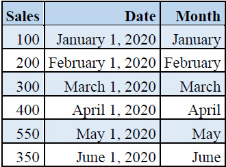
The Financial Analyst received data exported from the company’s Salesforce database containing sales data by month. The data is in columnar format vertically but it is needed horizontally.

Solution – Method with Formula

Setup the transpose formula. Select the array table. Use control + shift+ enter once you have selected the array table and the date will be presented horizontally as shown below.

Solution – Method Without Formula:

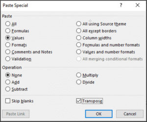
As an alternative, you can copy the data from the original table, and paste special values while clicking the transpose checkbox. This works, but will not automatically update the table if changes are made to the original table.

Overall, using the transpose function rather than doing a manual transpose method is a better method because it is automatically going to update things for you rather than going through the process of pasting special values.

I hope that helps. Please leave a comment below with any questions or suggestions. For more in-depth Excel training, checkout our Ultimate Excel Training Course here. Thank you!